
From Hillshade to Shaded Relief
Science, Art & ... Python
Producing quality shaded relief is no easy task. A good number of cartographers mastered hand drawing techniques of depicting terrain.
Methods have been developed, such as the "Swiss Style" whose pioneers, Fridolin Becker and Eduard Imhof have had far reaching influence in the area of relief representation. Their method uses oblique illumination from the upper left side, perspective hypsometric tints, contour lines and rock drawings and dismissed any other approach.
In the last few decades many cartographers applied Imhof's techniques with a variety of computer software. Notable would be the work of Ernst Spiess, Tom Patterson and Bernhard Jenny, to name just very few. Lately, several professionals in the field started to explore ways of using programming and scripting techniques to produce shaded relief tiled basemaps for web mapping.
Although I have studied and appreciated Imhof's and other cartographers' work, my own approach incorporates elements of art, mostly the ways in which form is represented with the use of tone, light and shadow.

Eduard Imhof, “Mount Everest”.

Tom Patterson, “Elemental Yosemite”.
It has become very facile to produce "shaded relief", one can easily create a hillshade, overlay hypsometric tint and–voilà!– shaded relief. And it doesn't look too bad. But there is a lot more to it than that.

Automatic "shaded relief".
Method
Here I am showing how I create shaded relief for print or screen maps and atlases, with perhaps a future part two, dedicated to web maps and tiles. The project and all the source code can be found on GitHub.
The smallest resolution of a typical map is 2048x1536 px, the size of an iPad with Retina display. For print the size could go as high as 5400x3600 px for a magazine spread and even higher for atlases and wall maps. The shaded relief component is created with GIS software, post-processed in Adobe Photoshop then used a a base layer in Adobe Illustrator, where the final map is assembled. I use Python to download DEM data and derive the slope, aspect and hillshade files to be used in desktop GIS software to output the shaded relief.
Conceptually, these are the elements we'll use:
Shape toning
The tone or value of the color is related to the angle between the ray of vision and the surface, ranging from the lightest – where the ray is perpendicular, to the darkest – where the ray is tangent to the surface.

Shaping form.
Direct illumination
Illumination will add highlight, midtone and shadow zones, as well as cast shadow. The consensus is that light should come from the upper left side, irrespective of the geographical location. However, if the orientation of the terrain demands it, the direction of the light should change.

Light & shadow.
Atmospheric perspective
Although the difference in elevation may not be too great, low lands should be slightly darker than high.

Dorothy Nelson, High Sierra.
Sky view factor
This technique computes a value for each cell given by the portion of the visible sky "seen" from that particular location. It can also be thought of as the amount of indirect light received by each cell.

Sky view factor.
Process
This workflow consists of creating the necessary file with Python and processing them within desktop GIS software to produce the shaded relief.
Action
Load DEM data
Check file (optional)
Reproject data (optional)
Resample data (optional)
Calculate slope
Calculate aspect
Calculate hillshade
Calculate cast shadow (optional)
Create colormap
Derive hypsometric tint
Create contours
Output files
Combine all images
Tools (libraries)
Python (os, elevation)
Python (numpy, gdal, matplotlib)
Python (rasterio, gdal, richdem, others)
Python (rasterio, gdal, richdem, others)
Python (numpy, matplotlib, richdem, others), GDAL
Python (numpy, matplotlib, richdem, others), GDAL
Python (numpy, matplotlib, richdem, others), GDAL
Python, GRASS, SAGA
(matplotlib)
(matplotlib)
OGR
Python (rasterio, gdal, os)
QGIS, ArcGIS
Python setup
# import modules
import os
import numpy as np
from numpy import gradient
from numpy import pi
from numpy import arctan
from numpy import arctan2
from numpy import sin
from numpy import cos
from numpy import sqrt
from numpy import zeros
from numpy import uint8
from osgeo import gdal
import rasterio
import elevation

# Numpy degree - radians conversions
deg2rad = 3.141592653589793 / 180.0
rad2deg = 180.0 / 3.141592653589793

# No data value for output
NODATA = -9999
Download data
This function uses the Elevation module to download 30m or 90m SRTM data. Needed arguments are the bounds, the name and the path of the DEM file to be writen.
# Function to download data
def download(w,s,e,n,name,path):
# create path to download and write file to disk
dem_file = path + name
# connect to site and get data
dem = os.path.join(os.getcwd(), dem_file)
# use the clip function of the elevation module to define bounds and output a GeoTIFF
# for 90m DEM use (product='SRTM3') as additional argument
elevation.clip(bounds=(w, s, e, n),output=dem)

# clean up stale temporary files and fix the cache in the event of a server error
elevation.clean()
return dem_file

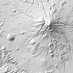
Shasta Mt. SRTM 30m, EPSG 4326.
Inspect, reproject and resample data
These steps are optional. Reprojecting at this stage could introduce banding with the slope and aspect calculations. I choose to leave the SRTM file in the original projection (EPSG 4326) throughout the Python stage and address it with the desktop app. In this case I worked on the 30m resolution but resampling may be necessary if the DEM's resolution is not appropriate for the scale of the map. I also tested the 90m SRTM of the same geographic extent, to compare the level of detail.
 Shasta Mt. SRTM 30m.
 Shasta Mt. SRTM 90m.
Inspect
These steps .
  # Function to download data
  def download(w,s,e,n,name,path):
  # create path to download and write file to disk
  dem_file = path + name
  # connect to site and get data
  dem = os.path.join(os.getcwd(), dem_file)
  # use the clip function of the elevation module to define bounds and output a GeoTIFF
  # for 90m DEM use (product='SRTM3') as additional argument
  elevation.clip(bounds=(w, s, e, n),output=dem)

  # clean up stale temporary files and fix the cache in the event of a server error
  elevation.clean()
  return dem_file


Caption.


